Think out of the box! Usually numbers that are formatted as text aren’t picked up or text values that have leading or.
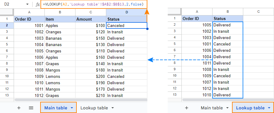
Vlookup In Google Sheets With Formula Examples - Ablebitscom
You're missing your search key, the first argument, and your index, the third argument, is incorrect.
Why is my vlookup not working in google sheets. From experience working with large spreadsheets from different sources, a common error that banes vlookup is having numbers that are formatted incorrectly or dirty data. When i copy and paste data into a column the vlookup doesn't auto update. The image below shows such a scenario.
The formula that i am using currently is =vlookup(a2,'form responses 1'!b$2:d,3) where a2 is the name of the person, form responses b$2:d refers to the first sheet, and 3 being the column where the hoodle/crew information is stored. Date joined (only entered if new and joined during. I have the work book set to auto calculate, and i've tried shift + f9, and ctrl + alt + shift + f9.
For this, we instruct the vlookup formula to search for the order number in a2 on the east sheet and return the value from. The quantity was in column 3, but after a new column was inserted it became column 4. As of february of 2020, this is not supported yet.
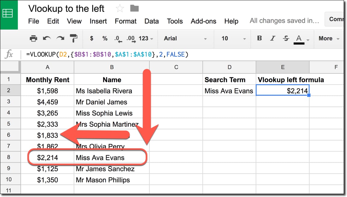
It seems that vlookup will not work properly without setting the 'is_sorted' argument; For example, you can search for the number 42, the word “cats”, or the value in cell b4. Google sheets vlookup cannot look at its left, it always searches in the first (leftmost) column of the range.
Vlookup is very common, popular and widely used function in excel and google sheets. How do we create a vlookup to the left? For example, if you have a sheet that collects form responses, you probably don’t want to be mucking it up with some analysis.
The vlookup function is a super popular formula but suffers from a major drawback. Vlookup will only look for a closest match to a value (by default) or an exact value. How to use vlookup in google sheets.
Vlookup also assumes by default that the first column in the table array is sorted alphabetically, and suppose your table is not set up that way, vlookup will return the first closest match in the table, which may not be the data you are looking for. Hi there i know this solution is not pretty, but i thought it would be a quick way to work out my club's subs payments which are coming up shortly for the new year. However, there’s a sneaky trick that lets us vlookup to the left, so we can search for a term and return a result from a column to the left of the original search column:.
The only way i can get the vlookup's to work is to click into the cell containing the data and press the enter key. The problem with a normal vlookup is that it only searches down the first column. Hi mark, before using an importrange () nested inside another function, you first have to allow access to the sheets to communicate with one another.
The problem that i keep getting however is that if the result of the vlookup is a cell with a hyperlink, the hyperlink does not work. If a new column is inserted into the table, it could stop your vlookup from working. You can’t lookup data to the left!
I will try to explain the main reasons one by one and how to address them. The help says that this is optional. Show paid yes or no (shows a yes or a no) col s:
First, we are going to pull the items. There may be several reasons for these common vlookup errors in google sheets. Because this is entered as an index number, it is not very durable.
The function is not returning correct values for all of the names. This is because of some limitations with the vlookup function, and sometimes. I have a spreadsheet with members details in and i've added a few columns showing:
I don't understand why it says that the date is not found. When i used references to numbers it would work. You may have forgotten that the vlookup function in google sheets always searches in the first (leftmost) column of the lookup range.
If the values for the search_key argument are in the second or some other column, vlookup won't work and will return the #n/a error: You currently have your range, the second argument, as b2:b, which is only 1 column, so your index cannot be greater than 1. Some names which do appear on sheet 1 are showing up as having nothing and even some.
You get an error when you try to do that. Paid 2008 (blank if no, 1 if yes) col r: Below is the summary table that we want to populate with the item names and amounts by looking up the order number in west and east sheets:.
One of my favorite things about google sheets, is that you can easily pass data across different sheets. I've entered some test text in i19, and the formula on monitoring, in o21 is now showing results. Other than these, it’s important to address the cause of wrong results in the vlookup output due to the accidental mistakes that we make.
=vlookup (f3, {d2:d5,b2:c5},3,0) for the left side aka reverse vloolup, the best formula to use in google sheets is vlookup itself! To do a left vlookup, use google sheets index match formula. These are the 2 sheets referred to in the formula.
In practice, we often forget about this and end up with vlookup not working because of the n/a error. As excel released the xlookup for most of the users now ( if you don’t have xlookup in your excel see here why ), many users are asking what happens if you try to open a file that has an xlookup formula in google sheets. The arguments of the vlookup function are:
Through vlookup function i could create a new table of which i create a pivot table which i can then easily refresh by pressing “refresh all” after i entered new data in “input”. Every time that i tried to use a string or a cell reference to a string for the 'search_key' it would not work. The easiest way to get the sheet to prompt you for that access is to do a single importrange () call on it own somewhere first.
But the majority of users complain that vlookup is not working correctly or giving incorrect results. If so, you'll need to update your vlookup ().
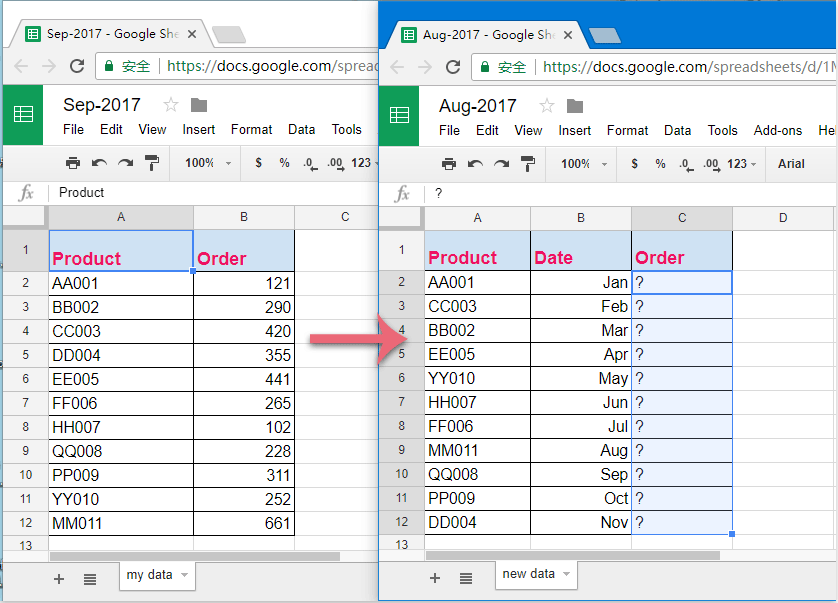
How To Vlookup Matching Value From Another Google Sheet
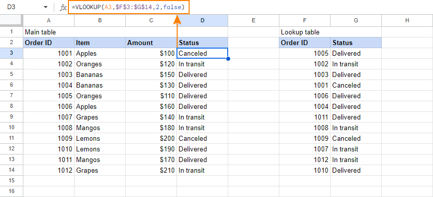
Vlookup In Google Sheets With Formula Examples - Ablebitscom
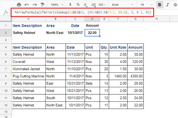
How To Use Vlookup With Multiple Criteria In Google Sheets Solved
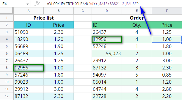
Trap And Fix Errors In Your Vlookup Formula In Google Sheets - Ablebitscom
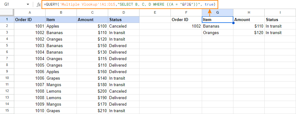
Vlookup In Google Sheets With Formula Examples - Ablebitscom
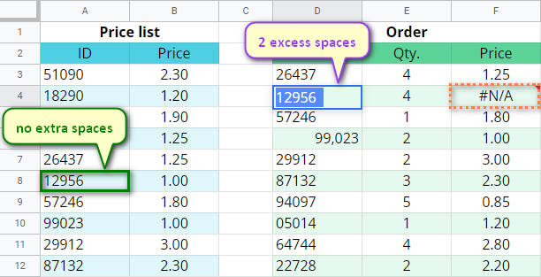
Trap And Fix Errors In Your Vlookup Formula In Google Sheets - Ablebitscom
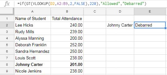
If Vlookup Combination In Google Sheets - Example Formulas
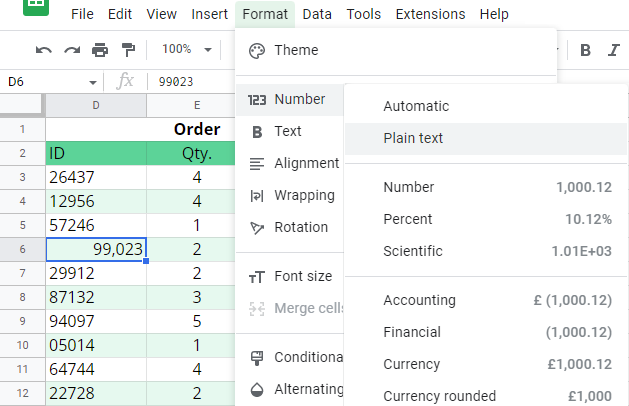
Trap And Fix Errors In Your Vlookup Formula In Google Sheets - Ablebitscom
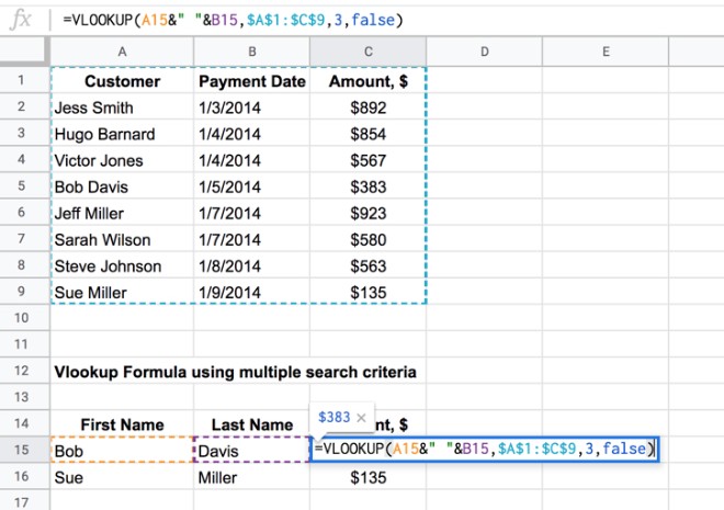
How To Vlookup Multiple Criteria And Columns In Google Sheets
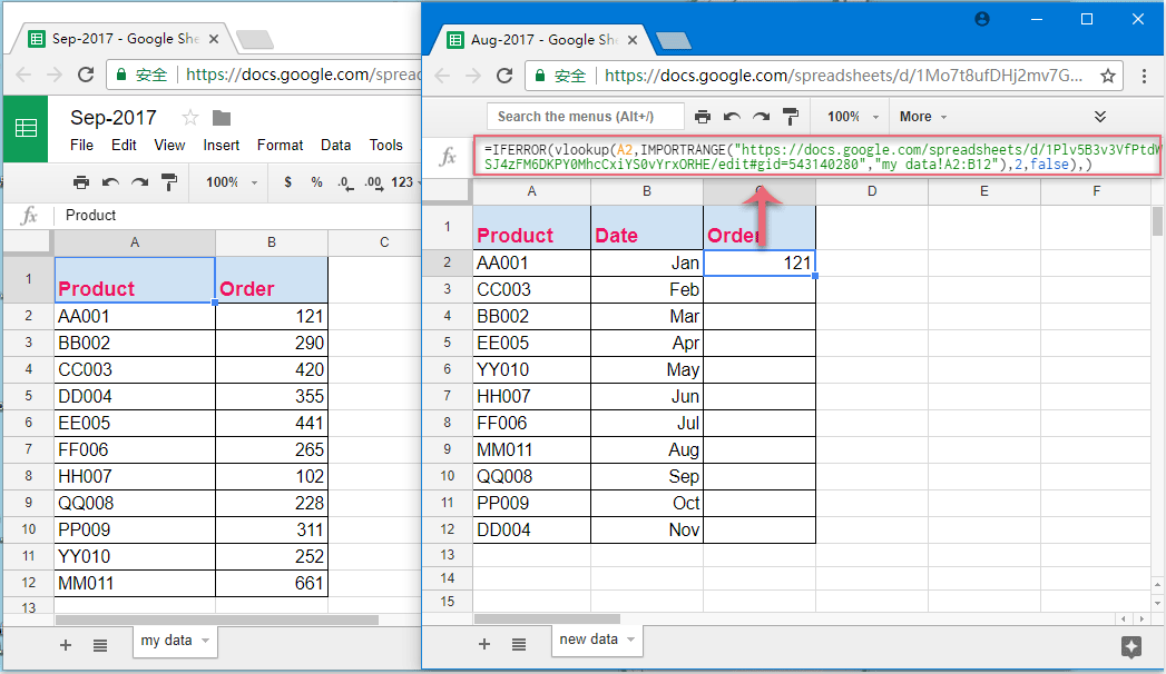
How To Vlookup Matching Value From Another Google Sheet
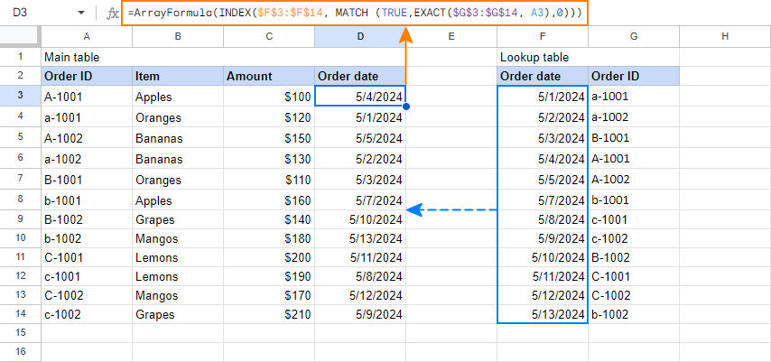
Vlookup In Google Sheets With Formula Examples - Ablebitscom
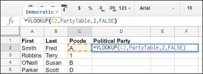
Quick Start Tutorial Vlookup Google Sheets Practice File
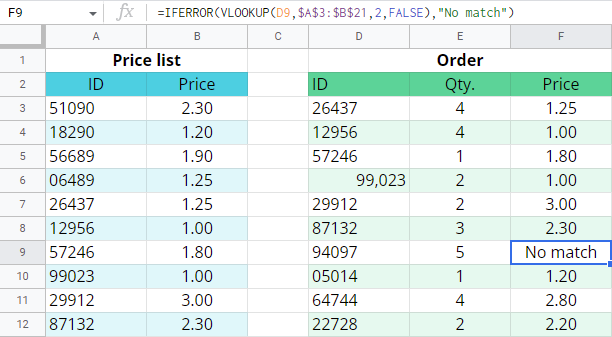
Trap And Fix Errors In Your Vlookup Formula In Google Sheets - Ablebitscom
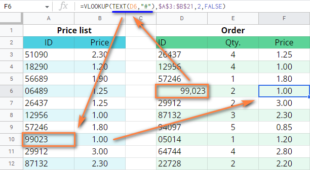
Trap And Fix Errors In Your Vlookup Formula In Google Sheets - Ablebitscom
How To Vlookup To The Left In Google Sheets -
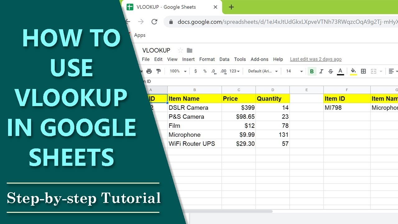
Vlookup Google Sheets How To Use Vlookup In Google Sheets Retrieve Data From A Cell - Youtube

Trap And Fix Errors In Your Vlookup Formula In Google Sheets - Ablebitscom
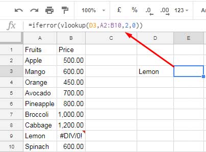
If Vlookup Combination In Google Sheets - Example Formulas
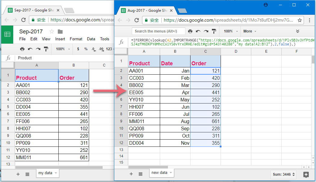
How To Vlookup Matching Value From Another Google Sheet
Comments
Post a Comment